Gazebo Simulation
Continuing our concept design, in this post we'll take our URDF from the previous tutorial, drop it into the Gazebo simulator, and drive it around!
Spawning our robot in Gazebo
Now that we have the rough shape of our robot worked out, it’s time to get it up and running in the Gazebo simulator.
Let's start by spawning our robot into Gazebo as-is, and we'll recap the important parts of the Gazebo overview tutorial while we're at it.
Launch robot_state_publisher with sim time
When we are running nodes with a Gazebo simulation, it's good practice to always set the use_sim_time parameter to true, which ensures that all the parts of the system agree on how to count time and can synchronise properly. This includes robot_state_publisher, so whether we run it directly (with ros2 run) or with our launch file (rsp.launch.py) we should make sure we set that parameter.
Launch robot_state_publisher with sim time using the following command (substituting your package name for my_bot):
ros2 launch my_bot rsp.launch.py use_sim_time:=true
Now it should be running and publishing the full URDF to /robot_description.
Launch Gazebo with ROS compatibility
If you haven't already installed Gazebo, you can do so using sudo apt install ros-jazzy-ros-gz.
Next up we need to run Gazebo, using the launch file provided by the ros_gz_sim package.
ros2 launch ros_gz_sim gz_sim.launch.py gz_args:=empty.sdf
This should open an "empty" Gazebo window. Make sure you tell it to use the built-in empty.sdf world which is a big flat plane - if you leave it actually empty there will be no ground and your robot will fall down!
Spawning our robot
Finally, we can spawn our robot using the create program provided by ros_gz_sim. Run the following command to do this (the entity name here doesn't really matter, you can put whatever you like). I also like to spawn the robot a little in the air (positive Z axis) to make sure it doesn't clip through the floor.
ros2 run ros_gz_sim create -topic robot_description -name my_bot -z 0.1
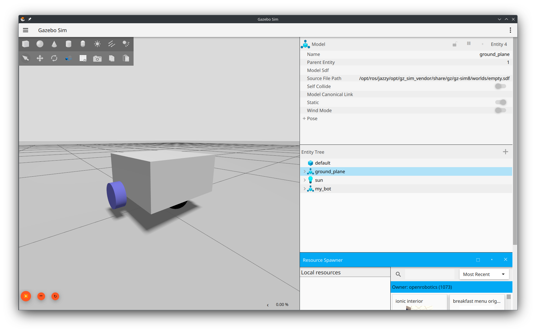
We should now see our robot appear in the Gazebo window. We can't drive it just yet, but that's ok, we'll fix that soon.
Simulation improvements
Creating a launch file
Our first improvement will be to create a launch file for running the simulation, to avoid having to close and rerun all three of these programs every time we make a change.
Create a new file in your launch/ directory called launch_sim.launch.py and paste the contents of the code block below.
Make sure you change the package name (line 21) to whatever you have called your package!
1
Take a minute to read through the file and get a general understanding of what it does (you don't need to understand every word right now). In this file we:
- "Include" the
rsp.launch.pyfile, from our package, and forceuse_sim_timeto be true - Declare a launch argument
worldso that we can change the simulated world - "Include" the Gazebo launch file (
gz_sim.launch.py), from theros_gz_simpackage with various arguments:-rstarts playback-v4increases loggingworldis our launch argument aboveon_exit_shutdowntells it to quit everything if Gazebo stops
- Run the
createnode fromros_gz_sim
After rebuilding and making sure all the previous programs have closed (including rsp.launch.py), we can try running this launch file. We should see our robot in Gazebo, exactly like before, only now we have an easier way get there.
ros2 launch my_bot launch_sim.launch.py
Note on gazebo tags
We saw in the Gazebo introduction tutorial that we can improve our Gazebo simulation by adding <gazebo> tags to our URDF file. Previous versions of Gazebo required us to add a <material> to every link for colours to work, but now it is able to use the colour from the URDF, so we only need <gazebo> tags when simulation-specific information must be added.
<link name="my_link">
    <!-- All the stuff that is inside the link tag -->
</link>

<gazebo reference="my_link">
    <!-- Gazebo-specific parameters for that link -->
</gazebo>

<gazebo>
    <!-- Gazebo parameters that are not specific to a link -->
</gazebo>
Some people like to create a whole extra xacro file for this to keep the simulation-specific stuff away from the core robot, but I like to keep them together so that it’s more obvious to me if I’ve written something contradictory (e.g. made the RViz and Gazebo colours different). It’s up to you what you want to do.
Friction
One important aspect of a good simulation is setting the friction parameters appropriately. For this particular robot you could skip this completely, or you could dive deep into tuning every detail of the simulation, but it's worth making at least this change.
We want to remove the friction on the caster wheel. We have modelled it as a fixed sphere but it is typically a smooth rolling surface, or very low-friction. Adding the following block below our caster_wheel link will disable friction in both directions, preventing it from dragging on the ground.
1
Something that always confused me was that the SDF spec mentions mu and mu2 as the friction settings (under some ode parameters), while lots of examples have mu1 and mu2. This is because the conversion from URDF to SDF expects the latter and converts it to the former. Speaking of friction in Gazebo, here is an interesting analysis which shows why it can be so confusing.
Torque & Velocity
Another change we will make is to limit the torque and velocity of our drive wheels. I've chosen 0.05 N.m for the effort (torque) and 10.0 rad/s for the angular velocity. You may choose to set your values higher (or lower), but without these, the simulation will respond instantly to changes which can feel a little "jerky". Note these changes are not inside a <gazebo> tag as the <limit> tag is part of the URDF spec.
1
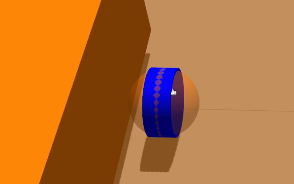
Spherical Collision
One last change to make is using a sphere as the collision geometry for our drive wheels. We can keep the radius the same as the cylinder we previously had, but now we have an infinitely small point of contact with the ground and will minimise weird odometry issues caused by the friction of the differential motion. (To see this in action, run Gazebo and RViz without this change and do a full rotation on the spot. While Gazebo gets back to its initial position, the RViz representation will be out-of-sync).
In our URDF we need to update the collision geometry (not visual!) for both the left and right links by replacing cylinder with sphere and removing the length parameter. The screenshot below was from the old Gazebo where you could more easily see the collision geometry, but you can do the same by toggling the collision geometry in the RobotModel in RViz.
1
If you have a better solution for this, I'd love to know!
Soon we'll actually drive our simulated robot to see if we got these right!
Controlling Gazebo via ROS
Understanding control in Gazebo
Before we start doing the work to get our robot driving, there are a couple of concepts we should take a moment to cover.
The first thing to note is that later on in the project we'll be using the fantastic ros2_control library to handle our control code.
What's cool about that is the same code will work for both the simulated robot AND the real robot, which minimises the differences between the two.
Since ros2_control is a bit complicated to set up, and the concepts surrounding it are worth spending time understanding well, for now we'll use a more simple differential-drive control system that comes with Gazebo, and just take a brief look at the concepts.
When we have a real robot, it will have a control system. The main thing that control system will do is take a command velocity input (how fast we want the robot to be going), translate that into motor commands for the motor drivers, read the actual motor speeds back out, and calculate the true velocity.
With ROS, that command velocity is on a topic called /cmd_vel, and the classic type is Twist, which is just six numbers - linear velocity in the x y and z axes, and angular velocity around each axis. For a differential drive robot though, we can only control two things: linear speed in x (driving forward and backwards), and angular speed in z (turning), so the other four numbers will always be 0. Newer systems like we will be using will usually use TwistStamped which adds the time stamp and reference frame.
Some of these diagrams require updating for newer versions but the overall principles are unchanged.

For some applications, like mapping, we are more interested in the robot position than its velocity. The control system can estimate this for us by integrating the velocity over time, adding it up in tiny little time steps. This process is called dead reckoning, and the resulting position estimate is called our odometry.
In the Gazebo overview tutorial, we saw that whenever we want to use ROS to interact with Gazebo, we do it with plugins. The control system will be a plugin (ros2_control or, for now, gz::sim::systems::DiffDrive) and that will interact with the core Gazebo code which simulates the motors and physics.

And this whole system then interacts with our diagram from the previous post. Instead of faking the joint states (with joint_state_publisher_gui), the Gazebo robot is spawned from /robot_description, and the joint_states are published by plugins. The plugins also broadcast a transfrom from a new frame called odom (which is like the world origin, the robot's start position), to base_link, which lets any other code know the current position estimate for our robot.

Adding control plugins
So to drive our robot around we'll need to add a control plugin to our URDF. Instead of putting more into our core file, we’re now going to create a new xacro file called gazebo_control.xacro, and add the include for it to our root file, robot.urdf.xacro.
After adding the XML declaration and robot tags, we want to add a <gazebo> tag, and inside that is where we’ll put our content.
1
Inside those <gazebo> tags, we will create a <plugin> tag to load the DiffDrive plugin. We also need to load the JointStatePublisher plugin to publish the joint states.
Copy and paste the whole plugin tag from below, and take a look through the various parameters:
- Check that the
Wheel Informationsection is correct (in case you used different measurements). - The
InputandOutputsections tell Gazebo how to interact with the ROS topics and transforms. Leave these alone for now.
You can see all the available tags at the DiffDrive API docs.
1
Bridge to ROS
In the new Gazebo, there is a whole separate set of topics that live internal to Gazebo and we need to bridge the data from there to ROS (and vice versa). We will add new file gz_bridge.yaml in the config directory which contains a list of topics that need bridging.
We specify:
- The topic name and type on the ROS side
- The topic name and type on the Gazebo side
- The direction it should map data
We also need to edit our launch_sim.launch.py file to launch the bridge node (called parameter_bridge) with our config.
1
Take a moment to review each entry in gz_config.yaml and understand why it is included, as well as the launch file changes.
Testing control
If we relaunch Gazebo now, our robot will be sitting there, ready to accept a TwistStamped command velocity on the /cmd_vel topic. The easiest way for us to produce that is with a tool called teleop_twist_keyboard.
To break down that name: teleop is short for teleoperation, i.e. remote operation by a human as opposed to autonomous control. Twist is the type of message ROS uses to combine the linear and angular velocities of an object. And keyboard is because we are using the keyboard to control it. However we actually want to use a TwistStamped (has the time and coordinate frame associated) for better compatibility with newer nodes.
Go ahead and run it using the following command:
ros2 run teleop_twist_keyboard teleop_twist_keyboard --ros-args -p stamped:=true -p use_sim_time:=true
That should produce the window below, with instructions on how to use it. If we start pressing the keys (e.g. i to move forward) then we should start to see the robot moving around.

Something you may find confusing/annoying/unintuitive about this tool is that it can only respond to input while the terminal window is active. It may be easiest to shrink the window down so that you can have it visible on top of your Gazebo window, and if you accidentally click away (e.g. to move the Gazebo camera) remember to switch back to the terminal.
A far more practical approach is to use a different package: teleop_twist_joy (specifically the teleop_node) which, combined with joy_node (from the joy package) gives the operator the ability to send command velocities using a controller, even when the terminal isn't active. We'll cover this in much more detail down the track when we dive deep into the control system, but if you're feeling adventurous you may want to experiment with it now.
Using our Simulation
Visualising the Result
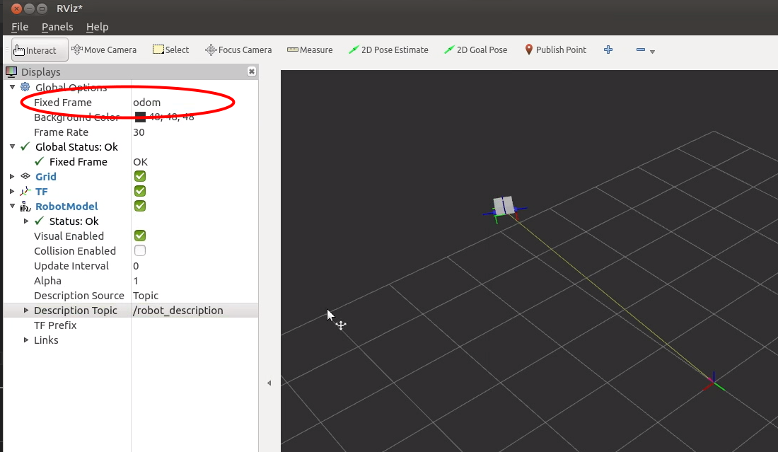
Now that we have our Gazebo plugin broadcasting a transform from odom to base_link, we should be able to see this in RViz.
Start RViz, and add the TF and RobotModel displays like in the last tutorial.
Now, set the fixed frame to odom. As we drive the robot around in Gazebo, we should see its motion matched in the RViz display.
The Problem with Plugins
I'm not sure whether the advice below is the "correct" way to deal with Gazebo plugins, but it's worth reading to avoid/understand crashes down the track!
Much of Gazebo's functionality is defined by plugins, many of which you can find listed here. How and when these plugins are loaded can be confusing. Here are a set of observations based on these two pages and my own testing that will hopefully help you to manage plugins well:
- As far as we are concerned, plugins can come from three different places: default config, world SDF, or robot URDF.
- There are three core plugins (
Physics,UserCommands, andSceneBroadcaster) which are loaded by default based on the file~/.gz/sim/8/server.config. If you manage to load a genuinely empty world, these plugins will be loaded. - When you launch Gazebo with a world file (SDF) to load, if that SDF has any plugins, even different to the default ones, then the default ones will not be loaded.
- If you spawn a robot after loading (even very quickly like we do), any plugins defined inside
<gazebo>tags in its URDF (which is converted at runtime to SDF) will be loaded in addition to the default or world plugins. - Certain plugins (e.g.
Sensors) cannot be loaded twice or it will kill Gazebo. Others (e.g.DiffDrive) seem to cope fine. - I don't think there is anyway to check if a plugin already exists before loading it (maybe a good feature in future?)
- The default
empty.sdfloads those default plugins explictly, but also theContactplugin, which I guess must be important? - Both the
filenameandnamefields of the<plugin>tag must be correct (I think in the old Gazebo thenamewas arbitrary).
Based on this, the approach taken in these tutorials is to ensure that at least following plugins are loaded in the SDF file:
<plugin filename="gz-sim-physics-system" name="gz::sim::systems::Physics"/>
<plugin filename="gz-sim-user-commands-system" name="gz::sim::systems::UserCommands"/>
<plugin filename="gz-sim-scene-broadcaster-system" name="gz::sim::systems::SceneBroadcaster"/>
<plugin filename="gz-sim-sensors-system" name="gz::sim::systems::Sensors"/>
<plugin filename="gz-sim-contact-system" name="gz::sim::systems::Contact"/>
Additional plugins can be loaded by the robot/s via their URDF when they spawn.
Making an Obstacle Course
Constructing a Gazebo world is outside the scope of this tutorial, but in short you want to:
- Add objects to your environment using the Resource Spawner
- Delete your robot using the Entity Tree so that it doesn't get included
- Use
Menu -> Save world as...to save the file as a.sdf - Edit that SDF to make sure the above plugin tags are all included
To load it back up we can supply the world path to our launch file. I store my worlds in a world directory so that when I launch from the workspace root it looks something like:
ros2 launch my_bot launch_sim.launch.py world:=src/my_bot/worlds/my_cool_world.sdf
See if you can make an obstacle course for your robot to drive around in!
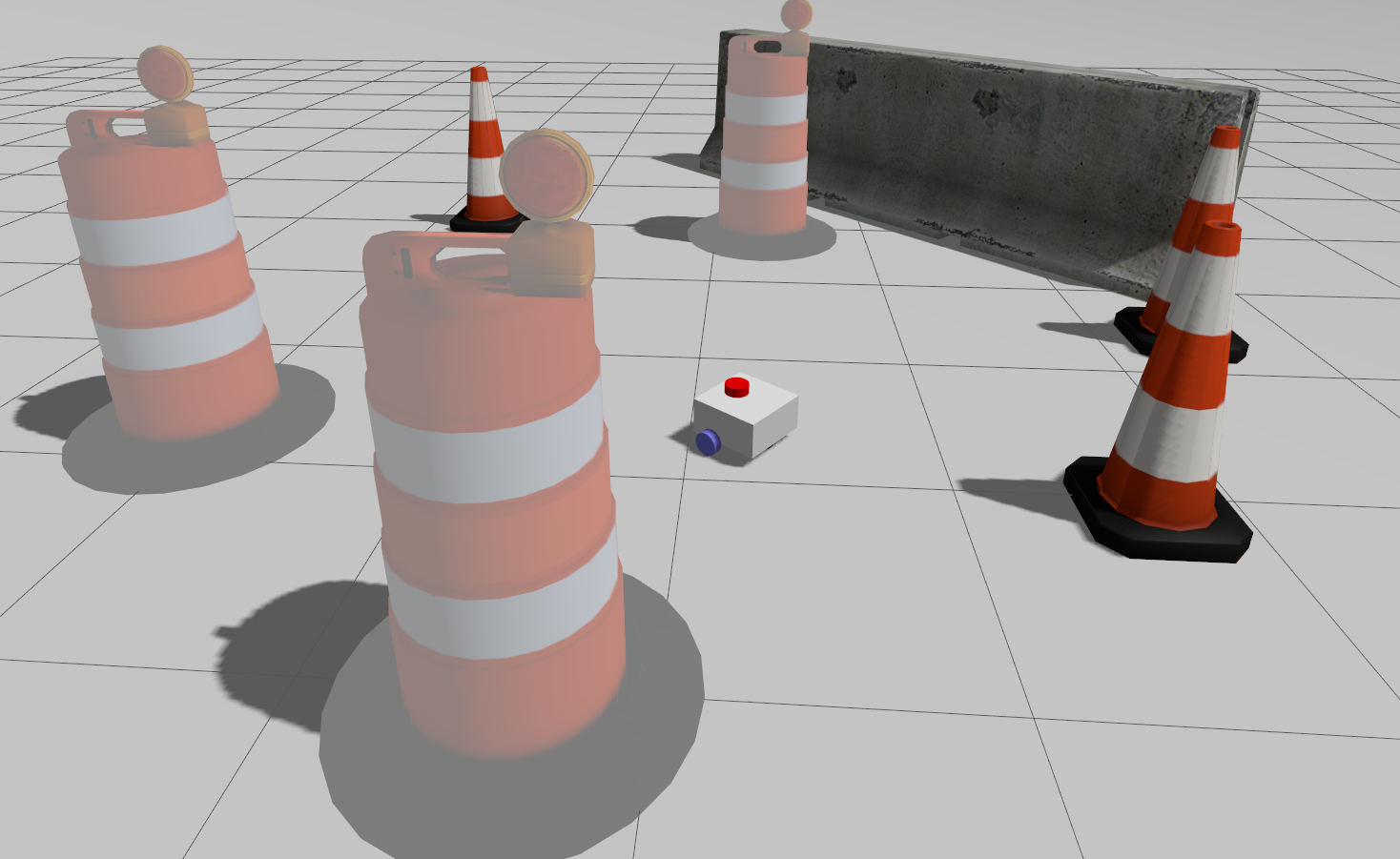
I really like the Construction Barrel, Construction Cone, and Jersey Barrier for making test worlds, but these appear washed-out in the new Gazebo. There is a way to fix this per-computer by modifying ~/.gz/fuel/fuel.gazebosim.org/openrobotics/models/construction cone/3/meshes/construction_cone.dae but it is a bit annoying. If anyone knows how to raise this with the appropriate author that would be appreciated!
Dealing with problems
Beyond the general Gazebo issues, there are a couple of things to check if the robot isn't driving quite right:
- Use
ros2 topic list,ros2 topic echo /cmd_vel, andros2 topic info /cmd_vel(or other topic names) to check the data is there and has sensible speeds etc. - Use the
Topic ViewerandTopic Echobuilt-in to Gazebo (three dots in the top right) to check the internal simulation data is correct - Make sure your inertia values are sensible, especially the masses
- Play around with the friction settings
- Check that the plugin parameters all make sense, especially the wheel separation and diameter
Up Next
Now that we have a broad design of our robot, and a working simulation, we can start figuring out the hardware side of things. In the next post we'll look at the brains of the robot - the Raspberry Pi.
Make sure you push your repo to git now so that you can pull it down onto the robot in the next tutorial!