ros2_control on the real robot
In the last tutorial we used ros2_control to drive our robot in Gazebo, but this time we're going to step things up and drive our robot in the real world. It won't make much sense if you haven't read the last tutorial, so make sure you do it first!
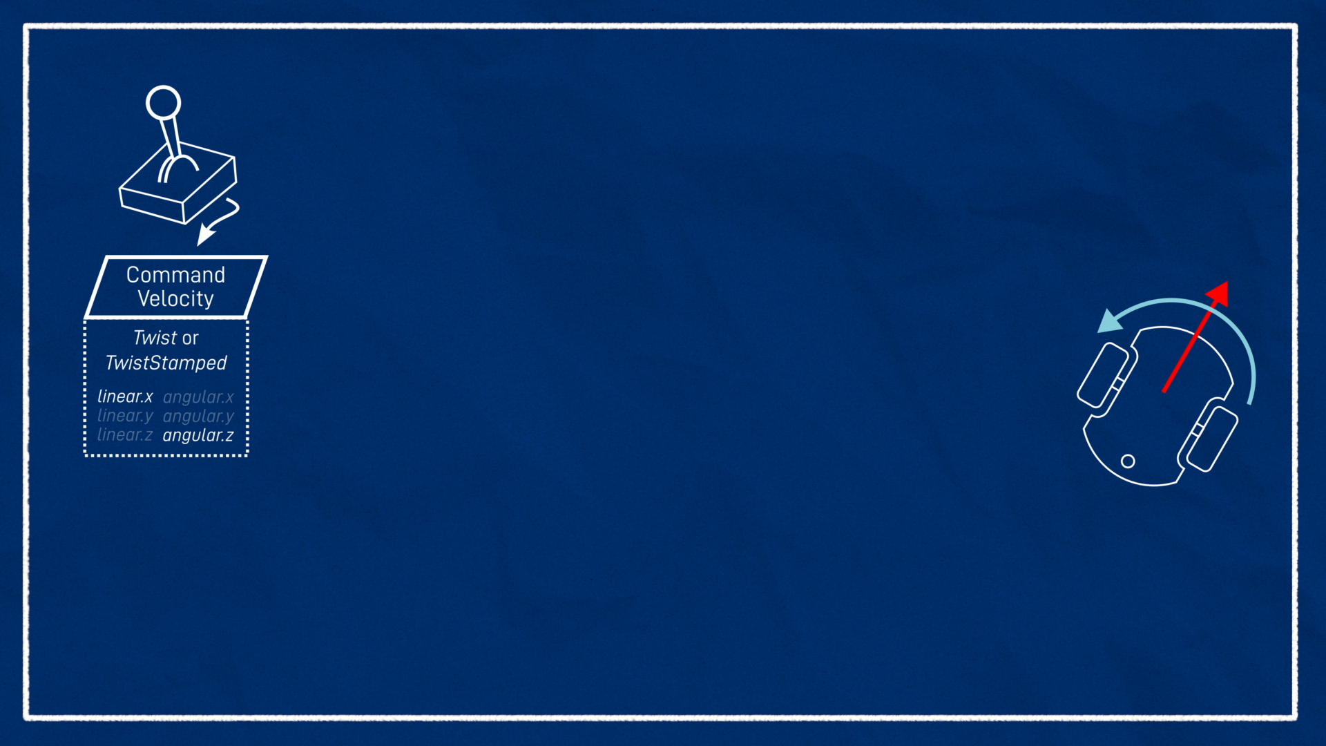
Before we dive into the code, let's quickly recap how ros2_control will work with our robot. At one end, we have a body velocity request, that's the velocity we want the robot to be moving through space, and we call this the command velocity. This could come from an operator, or something like a navigation stack. At the other end, we’ve got the physical robot, with two drive wheels, each of which are velocity controlled.
The command velocity is going to be a ROS topic of type TwistStamped (a 6-dimensional velocity) but since this particular robot’s motion is constrained to move forwards and backwards in X, and rotate around Z, we'll only use two of the values (linear.x and angular.z).
The tool we’re going to use to link up this command velocity to the actual motor velocities is ros2_control. This little ecosystem consists of three main parts:
- The
diff_drive_controllerplugin, provided byros2_controllers, which turns our command velocity into abstract wheel velocities - The hardware interface plugin, provided by us, which turns abstract wheel velocities into signals for the motor controller (e.g. via serial commands)
- The controller manager, provided by ros2_control, in this case using the
ros2_control_node, which links everything together
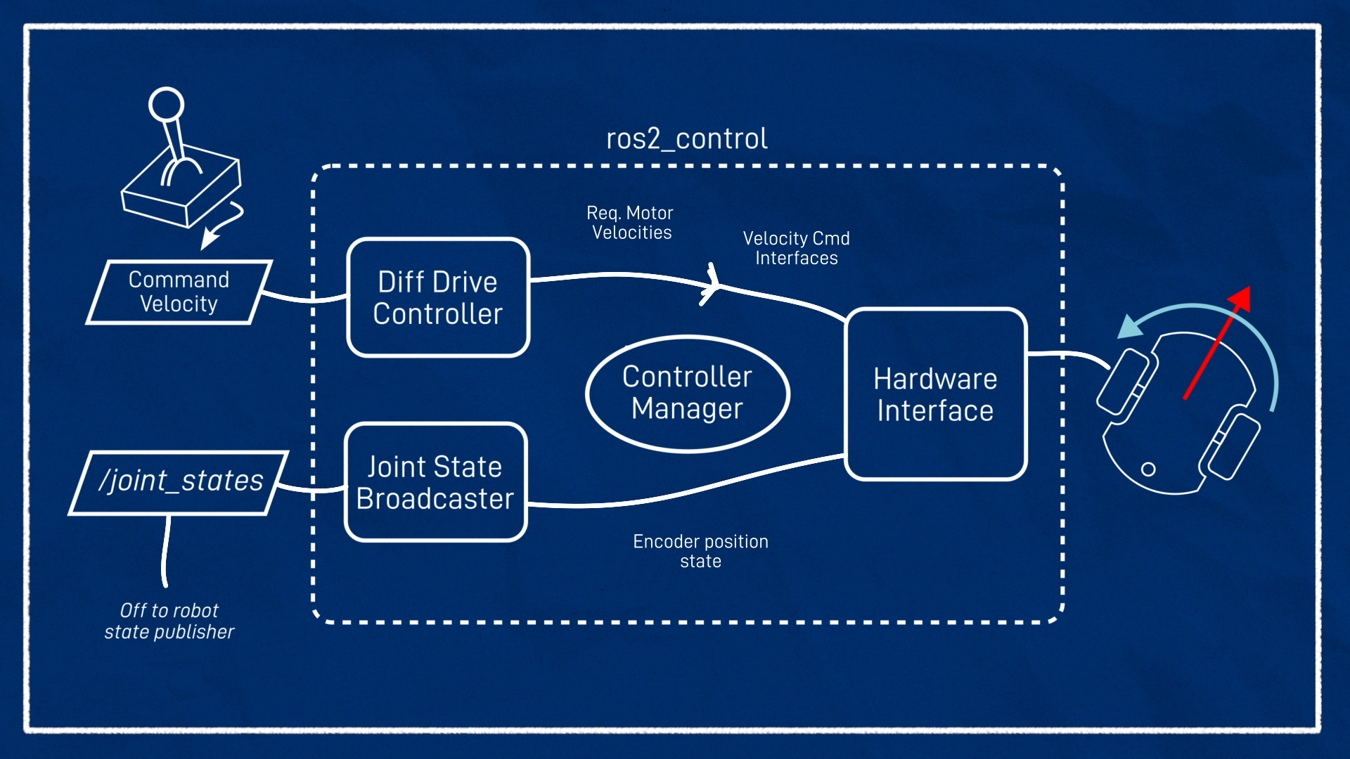
In addition to this, we have a controller called a joint state broadcaster. All this one does is read the motor encoder positions (provided by the hardware interface) and publish them to the /joint_states topic for robot state publisher to generate the wheel transforms. For this kind of robot it’s not strictly necessary but it makes the system “complete”.
In the previous tutorial we got all this working with a simulated robot, and a Gazebo-integrated controller manager, but this time we'll be doing it with a regular controller manager, our own hardware interface, on a real robot!
Getting the hardware interface
For this to work, we need a hardware interface for our robot. I've written one that you can use if you are using the same Arduino motor control code that I am, otherwise you'll need to find one online or write your own. Here's an example of one I found (have not tested) for Dynamixel motors.
Writing your own hardware interface is out of the scope of this tutorial, but I have made a video about it.
My hardware interface is called diffdrive_arduino, and all it does is expose the two velocity command interfaces (one for each motor), and the velocity and position state interfaces. Underneath, it’s simply just sending those “m” and “e” commands over serial that we saw in the motor tutorial (which never got a written version...oops!). Remember, the diff_drive_controller will be handling the actual control allocation.
It would be nice to be able to just sudo apt install diffdrive arduino but unfortunately we can’t do that. Originally this was because I depended on an unreleased package but that is no longer the case, so maybe some day? But you may want to modify the hardware interface anyway, so it's not a bad idea to compile it in your workspace.
To get the hardware interface we'll clone from my GitHub into our workspace and build it from source. It also needs a copy of the serial library it depends on, and to keep things simple I’ve made my own fork (of a different fork). So let’s hop onto the Pi and clone those into our workspace, then build them.
sudo apt install libserial-dev
cd robot_ws/src
git clone --branch humble https://github.com/joshnewans/diffdrive_arduino
cd ..
colcon build --symlink-install
Remember if you haven’t cloned your main project package onto the robot yet to do that one as well, and if you have already cloned it you'll want to pull the latest changes (from the last tutorial) from git.
Update the URDF
Now we need to update our URDF file to reflect the new hardware interface. Remember that we are editing these files on the Raspberry Pi.
To edit files on the Pi I like to use VS Code Remote Development. You can also just do it in the terminal with your favourite command line editor, or on your development machine and sync the files across to test them.
Let’s open up the ros2_control.xacro file we made in the last video. Here we will find the <ros2_control> block we wrote in the last tutorial to describe our hardware interface when we were using Gazebo, but now we need one for the real system.
FIrst up we need to add the ability to switch between the Gazebo ros2_control and the real ros2_control, this will be a similar system to the last tutorial where we switch between Gazebo ros2_control and pure Gazebo control.
We need to:
- Add another argument line in our main
robot.urdf.xacroand call itsim_mode, defaulted tofalse. - In
ros2_control.xacro, wrap the "real version" in<xacro:unless value="$(arg sim_mode)">, and the Gazebo version (uncommented) in<xacro:if value="$(arg sim_mode)">. - In
rsp.launch.py, expand our xacro command so that wheneveruse_sim_timeis true, we will be enablingsim_mode.
1
Now, whenever we are simulating, the Gazebo version should be enabled, and when we are running the live system the other one will be. Of course there are many <gazebo> tags throughout our URDF that we could disable when not in sim mode, but they will not be evaluated anyway so it doesn't really matter.
Then, to get the real one working, we need to add its configuration inside the <xacro:unless> block. The overall structure is similar to the Gazebo one, and the joint configuration is actually the same. The only real differences are in the <hardware> block where we load our real hardware interface and specify its parameters. We also give the whole thing a different name to keep it distinct.
Hardware interface plugins can expose a bunch of parameters for us to set. In this case we’ll have the following:
- Left and right wheel joint names
- Arduino loop rate
- Serial port
- Baud rate
- Comms timeout
- Encoder counts per revolution
You'll need to set the parameters appropriately for your system. The result should look something like:
1
Launch file
Now we need a launch file called launch_robot.launch.py. You can copy the one below, or copy your launch_sim.launch.py and remove all the references to Gazebo, sim time, and the ros2_control toggle (on the real robot we are always using it).
If you copy the one below, remember to change your package name!!!
1
I've highlighted some of those items to note, but this is a whole new file.
This launch file won't run correctly as-is, so don't bother trying.
Add the controller manager node
When using ros2_control we always need a controller manager running. In simulation, the Gazebo plugin starts it for us, but on the real robot we need to run it ourselves. Let's add a new node for it, and remember to add it at the end too.
We also need to pass it the path to our controller params file.
1
Previous versions of this tutorial (and the video) mention an alternative way to pass the robot description to the controller manager. The process for this is slightly different between Foxy, Humble, and Jazzy. This tutorial is for Jazzy and it should be detected automatically. It also dealt with some issues around use_sim_time which are no longer a problem.
Delaying our nodes
One problem we’ll run into is that we need the robot state publisher to have finished starting up before we run the ros2 param get command, or else we’ll fail to start the controller manager and nothing will work. The simplest (though probably not the best) way to do this is to simply add a time delay. The example below uses 3 seconds which should be enough.
1
We can also then delay the controller spawners until the controller manager has started. They do have a decent timeout anyway and so will probably be fine, but chaining it together like this is a bit neater.
1
Finally, we want to replace references at the end.
1
Ok, that should be all we need. Let’s rerun colcon to add the new launch file, and then we can test it!
Testing it out!
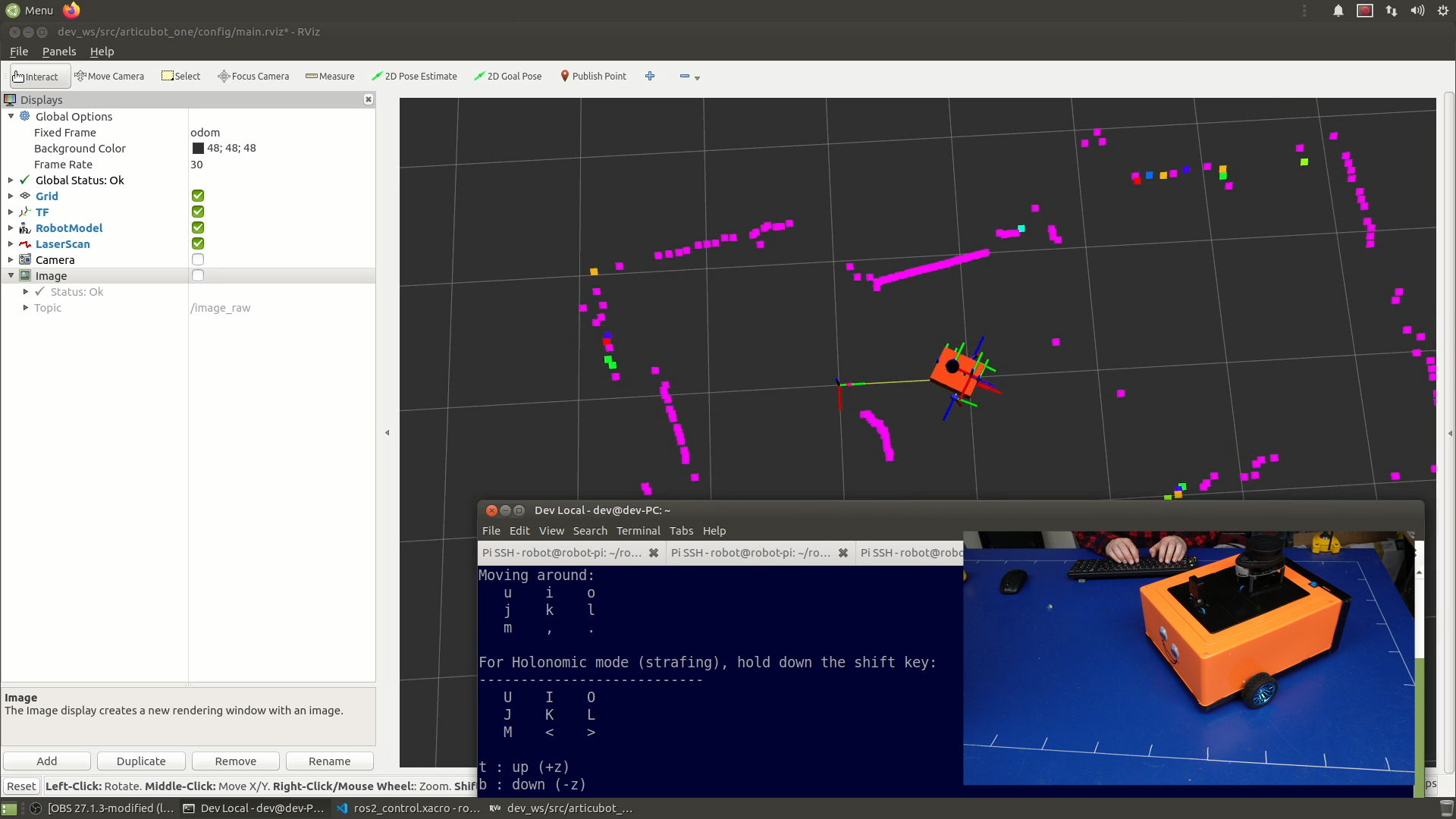
Basic driving
Make sure you prop your robot up before turning on the controllers for the first time, in case it sends incorrect values to the motors and sends the robot flying!
As a first test, we want to:
- Run our
launch_robot.launch.pyscript on the Pi, via SSH - Start RViz on our development machine, with the fixed frame set to
odomand various displays enabled (e.g. TF, RobotModel) - On the dev machine, run
teleop_twist_keyboard(or your preferred teleop method) with the topics remapped like in the previous tutorial (-r /cmd_vel:=/diff_cont/cmd_vel_unstamped)
As we send velocity commands, we should see:
- The wheels spinning in the expected direction
- The RViz display moving as if the robot were actually driving (it doesn't know the wheels are spinning in the air!)
- All the transforms etc. are displayed with no errors
If that seems to be working then it’s time to take the robot off its stand and try to drive it around! If you are finding that the wheel speeds are too fast/slow, the on-screen instructions for teleop_twist_keyboard show how to adjust them, however we'll look at some better approaches to teleop in the next tutorial.
Odometry accuracy
Now we want to see how accurate our odometry is. Odometry will never be perfect, which is why we use other localisation methods such as SLAM or GPS, but it is still worth getting as good as we can. There are three easy steps we can take to assess this (ensure they are done in order as each step is affected by the previous).
1. Encoder accuracy
- Prop the robot back up.
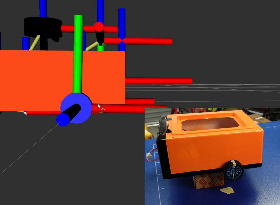
- Restart the controller so that the wheel axes are reset in RViz and note which way they are pointing (e.g. Y is pointing up).
- Set the RViz fixed frame to something robot-fixed (e.g.
base_link) - Put a marker (e.g. some tape) on the wheel.
- Drive forward for a while (e.g. 30 revolutions) and stop with the marker in the same spot
Your axes in RViz should be aligned the same as they were earlier. If it isn't, the encoder counts aren't being properly converted to angular measurements. Check that your counts-per-revolution are correct.
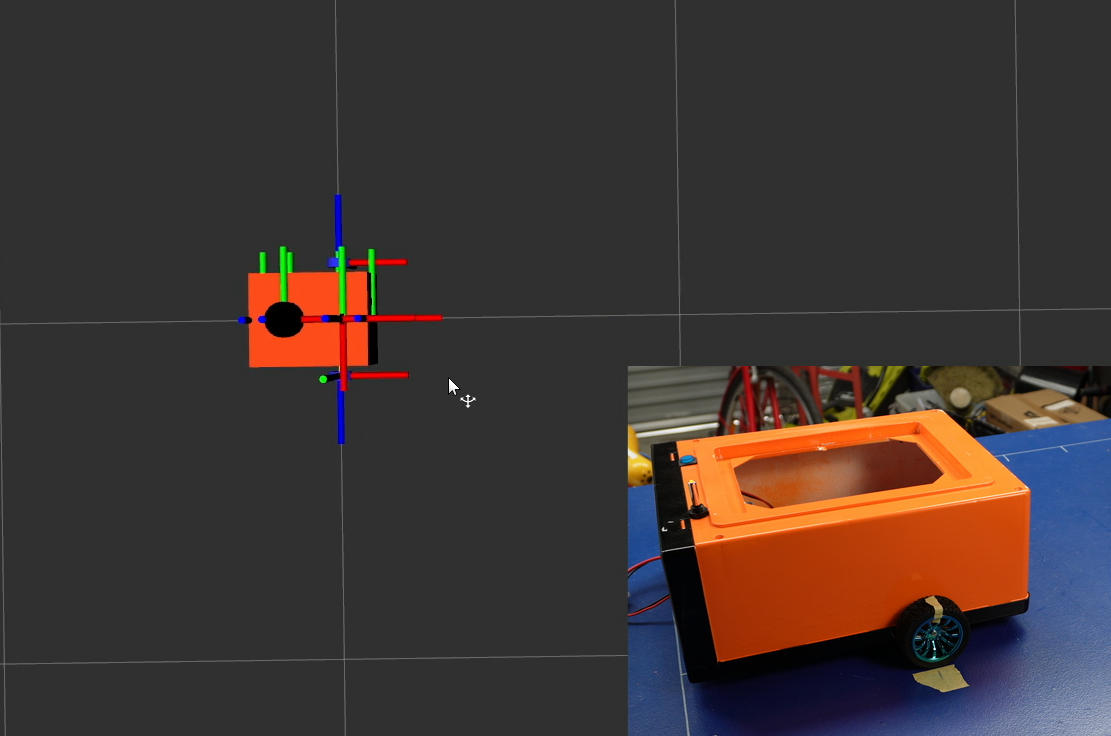
2. Wheel radius
- Place the robot on a large surface and note the wheel locations (e.g. with tape on the ground).
- Make another marker at a known distance ahead (e.g. 1m)
- Restart the controller so that the origin is reset in RViz (fixed frame doesn't matter too much but
odomis best) - Drive the robot until the wheels are aligned with the marker
The distance travelled in RViz should be the same as in real life. If not, you need to adjust your wheel radius.
3. Wheel separation
- Place a marker on the ground at the robot wheels
- Restart the controller to reset the robot orientation in RViz
- Drive the robot one revolution so that the wheels are back where they started
The robot should have turned exactly one revolution in RViz. If not, adjust your wheel separation.

Sensor Integration
This is also a chance to start testing our sensors (lidar, camera, and/or depth camera). We can simply run the launch files we created for these in previous tutorials.
We should see the laser data come up in RViz, and hopefully as we drive around, the detected objects should stay in approximately the same place. There will be some errors due to timing and also odometry drift.
Conclusion
Now we can drive our robot around which is a huge step forward, and hopefully it’s starting to feel like a real robot. In the next tutorial we'll look deeper at teleoperation (remote control), including how to control our robot using a game controller, or a smartphone.
Remember to push your changes!